Linear Regression Explained (Using R)

Linear Regression Explained (Using R)
by Curtis Murray - 17 July 2022
Introduction
I made this blog post to help introduce what linear regression is, why it’s useful, and how it works.
We’re going to see if we can find a relationship between the heights and weights of alien hippos on Mars.
There is a youtube video that I made in conjunction with this that you should also watch if you want!
Getting Things Set Up
Before we start any of the fun stuff, we need to get R set up!
Installing and Loading tidyverse
We’re going to be making use of a library called tidyverse, a collection of packages that are useful for data science.
To install tidyverse we can run the command below. Note that we only need to run this if we haven’t installed tidyverse before.
install.packages("tidyverse")This installs the package, but we can’t use it unless we load it up!
library(tidyverse)Loading in the Alien Hippo Data
Our data subjects are alien hippos on Mars.
As I mentioned previously, we’re interested to see if there is a relationship between their heights and weights.
To this end, I set sail to Mars, and recorded the heights and weights of 100 Martian hippos.
This data is convinantly stored in a CSV file online so that you don’t have to go to Mars to follow along. You can access the data like so, where we store it in a variable df.
df <- read_csv("https://raw.githubusercontent.com/curtis-murray/Teaching/main/LinearRegression/hippos.csv")The <- symbol is an assignment operator, which is just a fancy way of saying it’s the thing that lets you assign something to something. In this case, we’re assigning the variable name df with the data read in from the CSV file (read_csv) at the specified URL.
We can view df by calling it.
df## # A tibble: 100 × 2
## weight height
## <dbl> <dbl>
## 1 3920. 74.4
## 2 385. 9.58
## 3 -21.2 0.953
## 4 1178. 18.3
## 5 833. 15.9
## 6 2485. 45.4
## 7 2854. 54.8
## 8 3820. 72.9
## 9 713. 12.5
## 10 4360. 81.2
## # … with 90 more rowsThe output is a tibble with 100 rows and 2 columns. Each row corresponds to an individual Martian hippo, and the columns contain observation of their heights and weights.
Visualisation
Visualising the relationship between height and weight is an important first step in understanding their relationship.
To do this, we can make a graph. We will use the package ggplot2 to show a plot of the hippos’ heights on the x-axis and weights on the y-axis.
df %>%
    ggplot() +                                  # Create a ggplot
    geom_point(aes(x = height, y = weight)) +   # Add points for height (x-axis) and weight (y-axis)
    theme_bw() +                                # Styling
    labs(x = "Height (cm)", y = "Weight (kg)",  # Labelling
             title = "Alien hippo height and weight")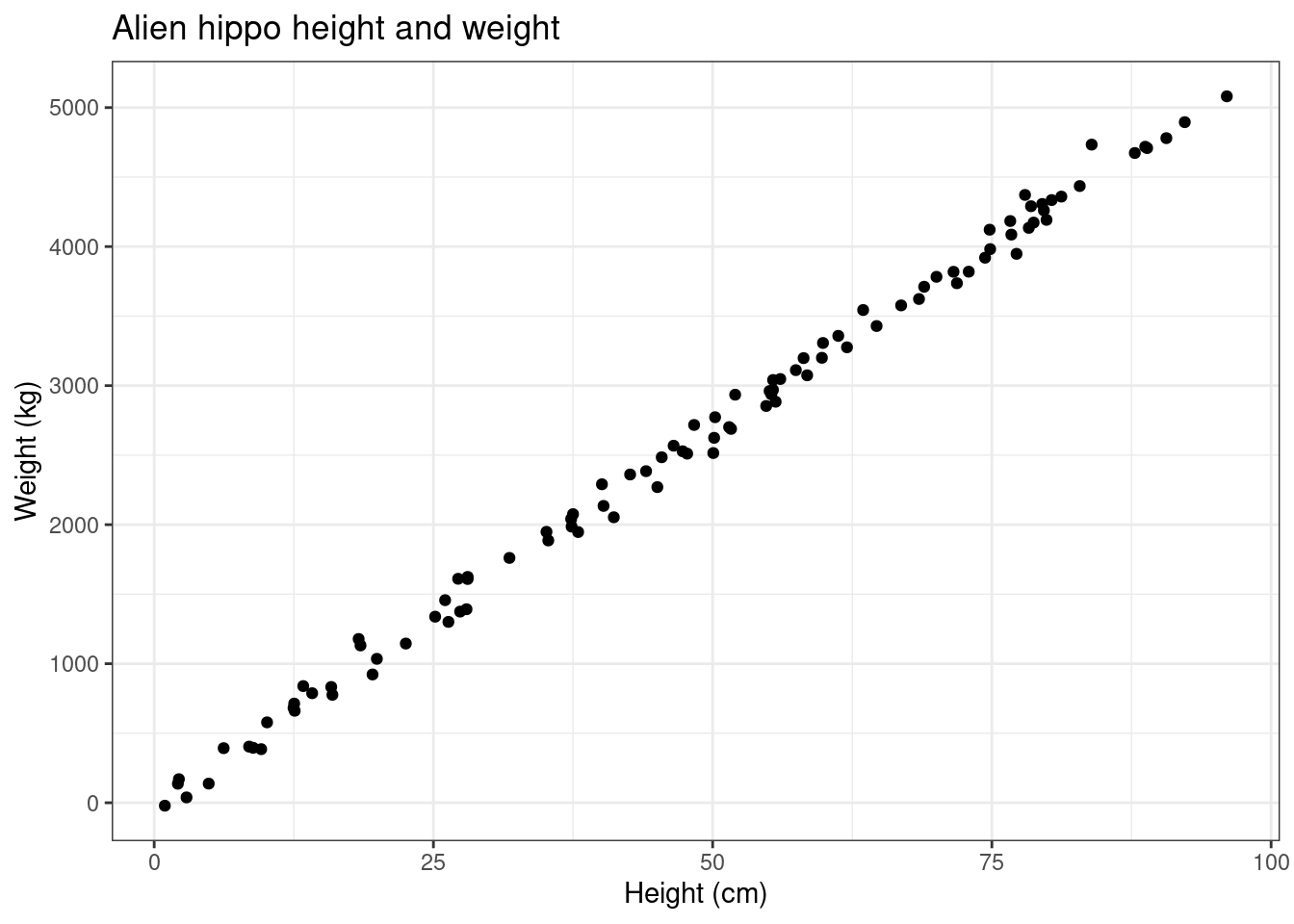
Each point on this graph corresponds to a hippo. We can see that there is some relationship between the height and weight of hippos. As the height increases, so too does the weight! How can we describe this relationship?
If we could find a function \(f\) such that, \[w = f(h),\] where \(w\) is weight, and \(h\) is height, then we could mathematically describe the relationship between height and weight!
Okay, but how do we find this function \(f\)?
Well, here it looks like the points form a straight line that passes through the origin.
This kind of relationship is quite simple, and can be formulated as;
\[\text{weight} \approx a \times \text{height},\] where \(a\) is a variable called the height coefficient. This wiggly equals sign \(\approx\) means “is approximately equal to”.
We don’t know what \(a\) is yet, but once we find it we will have a mathematical formulation for weight in terms of height.
To start, let’s do a bit of guesswork to work out what \(a\) should be.
Trial and Error
Instead of completely blindly guessing what \(a\) should be, let’s make a slightly informed guess. We can see that when a hippo’s height is approximately \(100\) cm, its weight is approximately \(5000\) kg.
Since we’re assuming \(0\) cm tall hippos are weightless, this means that for every centimetre increase in height, there is an estimated 50kg increase in weight. Then, our height coefficient \(a\) should be somewhere around \(50\).
\[\text{weight} \approx 50 \times \text{height}.\]
Let’s have a look at what it looks like for \(a\) between \(40\) and \(70\). We can change the value of \(a\) using the slider.
We can see that when \(a=40\), most of the points are above our line, and hence our relationship underestimates the weight. If we slide \(a\) up to \(70\) we now have the opposite problem! Our guess of \(a=50\) is a lot closer, but we can do better! Try out the slider, and see if you can find a value of \(a\) that makes the line fit best.
Okay, now that you’ve done this; what value of \(a\) did you find to make the line fit best? More importantly; how did you work out what it meant for the line to fit best?
We need some kind of metric that tells us how well the line fits. Actually, it turns out to be a little easier to define how badly the line fits; let’s do that!
First, we can find how badly the relationship or model fits the data.
We can look at what the model would estimate/predict the weights to be, and compare these estimates/predictions to their corresponding true weights. If we find the differences between the predictions and observations, we find the errors, i.e. how bad the model is at each point.
To see this visually, we highlight the errors as red dashes from observations to their corresponding predictions on the line. We want to get rid of as much red as possible!
We’re almost there! Now, we can summarise these errors into a single number to capture how badly model fits all the data.
To do this, we look at what is called the mean squared error, i.e. mean of the all of the squared error terms.
To help understand what this is, let’s define some terms and then make another plot.
We have that our observations are the heights and the weights. We can identify individual observations by using an indexing variable \(i\). The observation \((h_i,w_i)\) tells us the height and weight of the \(i^{\text{th}}\) hippo.
We can denote the weight predictions as \[\hat{w_i} = a\times h_i.\]
This allows us to then express errors, \(\varepsilon\) as \[\varepsilon_i = \hat{w_i} - w_i\]
And finally, the mean squared error \(MSE\) as \[ MSE = \frac{1}{n}\sum_{i=1}^n\varepsilon_i^2, \]
where \(n\) is the number of observations.
If this looks frightening, don’t worry, you can also just think of it as; \[ MSE = mean(\varepsilon_i^2).\]
Let’s take a look at what the mean squared errors looks like for our data.
Remember, the mean squared error is telling us how badly the model fits the observations. Since goodness of fit can be defined as the opposite of badness of fit, we want to find the value of \(a\) that corresponds to the minimum mean squared error, i.e. the model that is the least bad. This is also sometimes called the least-squares estimate.
Now you can see, if you thought \(53\) or \(54\) was the best value for \(a\), you were right! But can we do better?
We could improve the precision of our graph and continue with trial and error, but let’s try something even better!
Finding the Least-Squares Estimate through Calculus
Since we are interested in minimising the mean squared error, we can use calculus!
Remember that calculus allows us to find the rate of change, and, that local minima and local maxima occur when the rate of change is zero. So, all that we need to do is find when the rate of change of the mean squared error with respect to \(a\) is zero.
\[\begin{aligned} \frac{d}{da}MSE &=\frac{d}{da}\left[ \frac{1}{n}\sum_{i=1}^n\varepsilon_i^2 \right] \\ &=\frac{d}{da}\left[\frac{1}{n}\sum_{i=1}^n\left(\hat{w_i}-w_i\right)^2\right]\\ &=\frac{d}{da}\left[\frac{1}{n}\sum_{i=1}^n\left(a\times h_i-w_i\right)^2\right] \\ &=\frac{1}{n}\sum_{i=1}^n \frac{d}{da}\left[\left(a\times h_i-w_i\right)^2\right]\\ &=\frac{1}{n}\sum_{i=1}^n 2h_i\left(a\times h_i-w_i\right) \end{aligned}\]
Then, we set this to zero, and solve for \(a\).
First, \[ \begin{aligned} 0 &= \frac{1}{n}\sum_{i=1}^n 2h_i\left(a\times h_i-w_i\right)\\ &= \sum_{i=1}^n \left(a\times h_i^2-w_i\times h_i\right)\\ &=a\sum_{i=1}^n h_i^2- \sum_{i=1}^n w_i\times h_i\\ \end{aligned} \] \[ \begin{equation} a = \frac{\sum_{i=1}^n w_i\times h_i}{\sum_{i=1}^n h_i^2} \tag{1} \end{equation} \]
Equation (1) tells us exactly what the least squares estimate is for \(a\) using the weights and heights in a simple(ish) computation!
a_calc_method <- df %>%
  summarise(a = sum(weight*height)/sum(height^2)) %>%
  pull(a)

a_calc_method
## [1] 53.57613ggplot(df, aes(df$height, df$weight)) +
geom_point(aes(height, weight)) +
geom_line(aes(height, a_calc_method*height), color = "blue") +
theme_bw() +
labs(x = "Height (cm)", y = "Weight (kg)",
subtitle = "Alien hippo height and weight")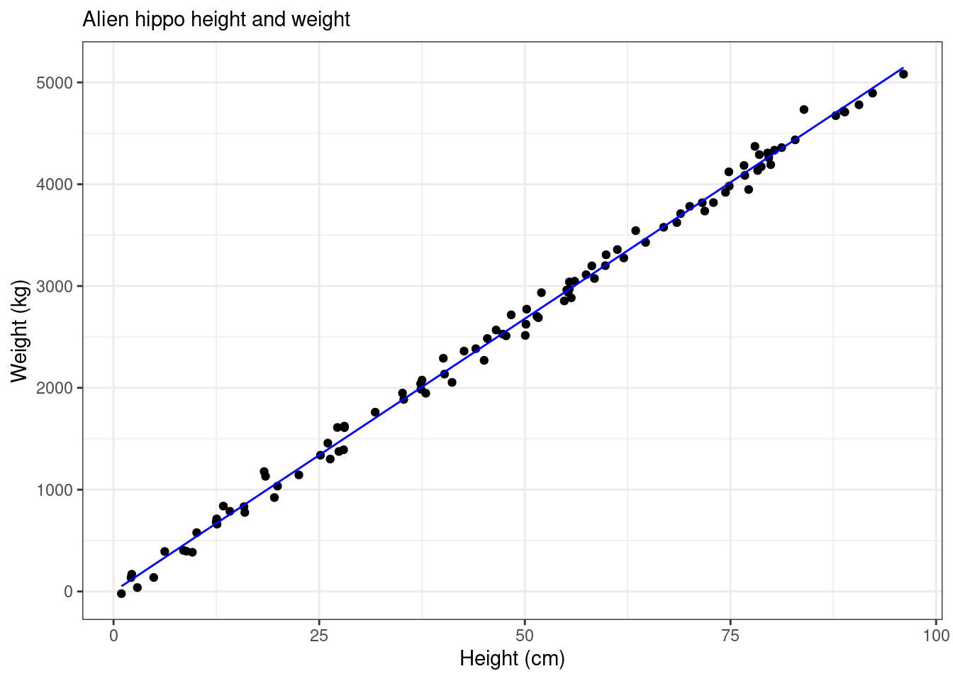
Linear Regression Using R
Now that we know how it works, we can cheat and use R to do the hard work for us!
All we have to do, is use the lm() function, and pass in the data and an appropriate formula.
model <- df %>%
  lm(formula = weight~height-1)

model
##
## Call:
## lm(formula = weight ~ height - 1, data = .)
##
## Coefficients:
## height
## 53.58model$coefficients## height
## 53.57613We can see that the result from R is the same as what is found using calculus!
Note that we use the formula
weight~height-1to show that weight is related to height, and there is no intercept term (this is the \(-1\) in the formula), as we are specifying that the data passes through the origin.
I hope this helped :) Remember to check out the Youtube Video.
- © Curtis Murray, 2022